Pair Modelled and Observed Data
One common analytical need is to obtain a combined data set of modelled and
observed observations at the same times and locations. This can be done using
the collect_inst_model_pairs() function in Match. This
routine takes a date range as input, and then extracts modelled observations at
the specified instrument location. However, it does not interpolate in time.
Details about the interpolation of modelled data onto the instrument location
can be found in the Extract routine,
extract_modelled_observations().
Match Data by Location
In the example below, we load a DINEOFs file created for testing purposes and pair it with C/NOFS IVM data. This is a global example for a single time, since in this instance DINEOFs was used to create a day-specific emperical model. Comparisons with output from a global circulation model would look different, as one would be more likely to desire the the closest observations to the model time rather than all observations within the model time.
This example uses the external modules:
pysat
pysatNASA
Load a test model file from pyDINEOFs. It can be downloaded from the GitHub
repository using the standard pysat.Instrument.download() method. We
will also set the model-data input keyword arguements that are determined by
the model being used. The DINEOFs test data applies for an entire day, so the
pair_method is 'all' and the time_method is 'max'.
import datetime as dt
from os import path
import pysat
import pysatNASA
import pysatModels as ps_mod

# Set the instrument inputs
inst_module = ps_mod.models.pydineof_dineof
inst_id = ''
tag = 'test'

# Initialize the model input information, including the keyword arguements
# needed to load the model Instrument into an xarray Dataset using
# the match.load_model_xarray routine
stime = inst_module._test_dates['']['test']
tinc = dt.timedelta(days=1)  # Required input is not used in this example
dineofs = pysat.Instrument(inst_module=inst_module, tag=tag, inst_id=inst_id)

# If you don't have the test file, download it
try:
    filename = dineofs.files.files[stime]
except KeyError:
    dineofs.download(stime, stime)
    filename = dineofs.files.files[stime]

# Set the input keyword args for the model data
input_kwargs = {"model_load_kwargs": {'model_inst': dineofs,
                                      'filename': filename},
                "mod_lon_name": "lon",
                "mod_name": [None, None, "lon", "lt"],
                "mod_units": ["km", "deg", "deg", "h"],
                "mod_datetime_name": "time",
                "mod_time_name": "time",
                "model_label": dineofs.name,
                "pair_method": "all",
                "time_method": "max",
                "sel_name": "model_equator_model_data"}
Next, get observational data to match with the model data. In this example, we will use C/NOFS-CINDI IVM data, since the DINEOFs test file contains meridional E x B drift values.
# Initialize the CINDI instrument, and ensure the best model interpolation
# by extracting the clean data only after matching.
cindi = pysat.Instrument(inst_module=pysatNASA.instruments.cnofs_ivm,
                         clean_level='none')

try:
    cindi.files.files[stime]
except KeyError:
    # Desired date not on filesystem, download missing data.
    cindi.download(stime, stime)

# Set the input keyword args for the CINDI data
input_kwargs["inst_clean_rout"] = pysatNASA.instruments.cnofs_ivm.clean
input_kwargs["inst_download_kwargs"] = {"skip_download": True}
input_kwargs["inst_lon_name"] = "glon"
input_kwargs["inst_name"] = ["altitude", "alat", "glon", "slt"]
With all of the data obtained and the inputs set, we can pair the data. It
doesn’t matter if the longitude range for the model and observational data
use different conventions, as the collect_inst_model_pairs() function
will check for compatibility and adjust the range as needed.
matched_inst = ps_mod.utils.match.collect_inst_model_pairs(
    stime, stime + tinc, tinc, cindi, **input_kwargs)
The collect_inst_model_pairs() function returns a
pysat.Instrument object with the CINDI and DINEOFs data at the
same longitudes and local times, after raising warnings for times and places
when the observed data location lies outside of the model interpolation limits.
The CINDI data has the same names as the normal pysat.Instrument.
The DINEOFs data has the same name as the normal pysat.Instrument,
but with 'dineof_' as a prefix to prevent confusion. You can change this
prefix using the model_label keyword argument, allowing multiple
models to be matched to the same observational data set.
# Using the results from the prior example
print([var for var in matched_inst.variables
       if var.find(input_kwargs['model_label']) == 0])
This produces the output line: ['dineof_model_equator_model_data'].
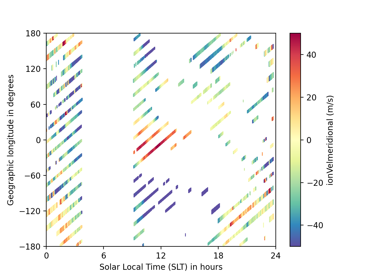
To see what the matched data looks like, let’s create a plot that shows the locations and magnitudes of the modelled and measured meridional E x B drifts. We aren’t directly comparing the values, since the test file is filled with randomly generated values that aren’t realistic.
import matplotlib as mpl
import matplotlib.pyplot as plt

# Initialize the figure
fig = plt.figure()
ax = fig.add_subplot(111)

# Plot the data
ckey = 'ionVelmeridional'
dkey = 'dineof_model_equator_model_data'
vmax = 50
con = ax.scatter(matched_inst['slt'], matched_inst['glon'],
                 c=matched_inst[ckey], s=matched_inst[dkey].abs() * 10 + 10,
                 marker='|', vmin=-vmax, vmax=vmax, lw=1,
                 cmap=mpl.cm.get_cmap('Spectral_r'))
cb = plt.colorbar(con, ax=ax)

# Format the figure
ax.xaxis.set_major_locator(mpl.ticker.MultipleLocator(6))
ax.yaxis.set_major_locator(mpl.ticker.MultipleLocator(60))
ax.set_xlabel(matched_inst.meta['slt', matched_inst.meta.labels.desc])
ax.set_ylabel(matched_inst.meta['glon', matched_inst.meta.labels.desc])
ax.set_xlim(0, 24)
ax.set_ylim(-180, 180)
cb_label = "{:s} ({:s})".format(
    matched_inst.meta[ckey, matched_inst.meta.labels.name],
    matched_inst.meta[ckey, matched_inst.meta.labels.units])
cb.set_label(cb_label)

# If you can display and are not running interactivly:
plt.show()
Match Data by Location and Time
For models with Universal Time variations over the desired period, you can also
match model and data results by both time and location. This is done by
setting the time_method keyword arguement to 'min'.