Extract Observational-Style Data

Comparison of model and Instrument data is supported in pysatModels, in part, by enabling the extraction (or interpolation) of model output onto the same locations as an observation-style data set. One common example is ‘flying’ a satellite through a model. The satellite locations are used to extract relevant model data enabling direct comparison of observed and modeled values.

Regular Grid Models

pysatModels.utils.extract.extract_modelled_observations() supports extracting values from models on a regular grid onto observed locations. The function can linearly interpolate model values onto instrument locations or use the nearest modeled location. Uses scipy.interpolate.interpn() as the underlying interpolation function. This function can handle either pandas or xarray formatted pysat.Instrument observational data. Because multi-dimensional data can be more complicated, let’s use Jicamarca ISR drift data as an example.

import datetime as dt
import pandas as pds
import pysat
from pysatMadrigal.instruments import jro_isr
import pysatModels

# Initalize the observed data
stime = dt.datetime(2021, 1, 3)
jro = pysat.Instrument(inst_module=jro_isr, tag='drifts', user='Your Name',
                       password='your.email@inst.type')

# Download data if necessary
if stime not in jro.files.files:
    jro.download(start=stime)

# Get fake model data from the pysat model test instrument
mod_drange = pds.date_range(stime, stime + dt.timedelta(days=1), freq='1D')
model = pysat.Instrument('pysat', 'testmodel', tag='',
                         file_date_range=mod_drange)
model.load(date=stime)

# Get the model longitude range, and make sure the loaded data has the
# same range
if model['longitude'].min() >= 0 and model['longitude'].max() > 180:
    min_lon = 0.0
    max_lon = 360.0
else:
    min_lon = -180.0
    max_lon = 180.0

jro.custom_attach(pysat.utils.coords.update_longitude,
                  kwargs={'lon_name': 'gdlonr', 'high': max_lon,
                  'low': min_lon})
jro.load(date=stime)

# Check the loaded variables, you may receive a warning for unknown data
# variables (this is ok).
print(jro.variables, model.variables)

This yields:

['time', 'gdalt', 'gdlatr', 'gdlonr', 'kindat', 'kinst', 'nwlos', 'range',
 'vipn', 'dvipn', 'vipe', 'dvipe', 'vi7', 'dvi7', 'vi8', 'dvi8', 'paiwl',
 'pacwl', 'pbiwl', 'pbcwl', 'pciel', 'pccel', 'pdiel', 'pdcel', 'jro10',
 'jro11', 'year', 'month', 'day', 'hour', 'min', 'sec', 'spcst', 'pl',
 'cbadn', 'inttms', 'azdir7', 'eldir7', 'azdir8', 'eldir8', 'jro14',
 'jro15', 'jro16', 'ut1_unix', 'ut2_unix', 'recno'] ['uts', 'time',
 'latitude', 'longitude', 'altitude', 'slt', 'mlt', 'dummy1', 'dummy2']

To extract the desired data points, you need to specify the model time variable names, the matching observation and model coordinate names and dimensions, the variables you want to select for extraction, and the extraction method. For this example, we’ll be matching the vertical drift from JRO ('vipn') to the fake model variable with the appropriate dimensions ('dummy2').

# Set the model dummy variable units
model.meta['dummy2'] = {model.meta.labels.units: 'm/s'}

# Get the xarray data from the model instrument, with metadata attached
model_data = pysatModels.utils.convert.convert_pysat_to_xarray(model)

# Set the extract input parameters
input_args = [jro, model_data, ["gdlonr", "gdlatr", "gdalt"],
              ["longitude", "latitude", "altitude"], "time", "time",
              ["deg", "deg", "km"]]
input_kwargs = {'sel_name': ['dummy2']}

# Run the extract function
added_vars = pysatModels.utils.extract.extract_modelled_observations(
    *input_args, **input_kwargs)

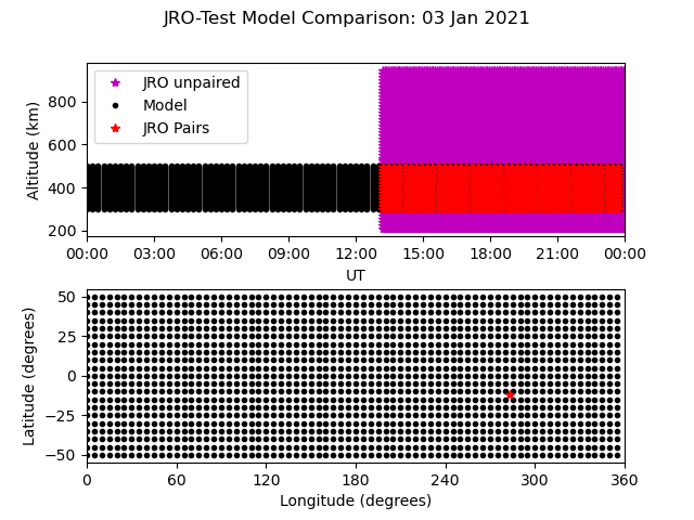
The output from this function will let you know the variable names that were added to the observational data Instrument. If we plot this data, we can visualize how the selection occurred.

import matplotlib as mpl
import matplotlib.pyplot as plt
import numpy as np

# Initialize a figure with two subplots
fig = plt.figure()
ax_alt = fig.add_subplot(211)
ax_loc = fig.add_subplot(212)

# Create plottable model locations
mlon, mlat = np.meshgrid(model['longitude'], model['latitude'])
mtime, malt = np.meshgrid(model.index, model['altitude'])

# Get the paired and unpaired JRO indices
igood = np.where(~np.isnan(jro[added_vars[0]]))
ibad = np.where(np.isnan(jro[added_vars[0]]))

# Plot the altitude/time data
ax_alt.plot(jro.index[ibad[0]], jro['gdalt'][ibad[1]], 'm*',
            label='JRO unpaired')
ax_alt.plot(mtime, malt, 'k.')
ax_alt.plot(jro.index[igood[0]], jro['gdalt'][igood[1]], 'r*',
            label='JRO Pairs')

# Plot the the lat/lon data
ax_loc.plot(mlon, mlat, 'k.')
ax_loc.plot(jro['gdlonr'], jro['gdlatr'], 'r*')

# Format the figure
ax_loc.set_xlim(0, 360)
ax_loc.xaxis.set_major_locator(mpl.ticker.MultipleLocator(60))
ax_loc.set_xlabel('{:} ({:})'.format(
    model.meta['longitude', model.meta.labels.name],
    model.meta['longitude', model.meta.labels.units]))
ax_loc.set_ylabel('{:} ({:})'.format(
    model.meta['latitude', model.meta.labels.name],
    model.meta['latitude', model.meta.labels.units]))

ax_alt.lines[1].set_label('Model')
ax_alt.legend(loc=2)
ax_alt.set_xlabel('UT')
ax_alt.set_xlim(stime, stime + dt.timedelta(days=1))
ax_alt.xaxis.set_major_formatter(mpl.dates.DateFormatter('%H:%M'))
ax_alt.set_ylabel('{:} ({:})'.format(
    model.meta['altitude', model.meta.labels.name],
    model.meta['altitude', model.meta.labels.units]))

fig.suptitle('JRO-Test Model Comparison: {:}'.format(
    stime.strftime('%d %b %Y')))
fig.subplots_adjust(hspace=.3)

# If not working interactively
plt.show()

And this should show the figure below.

pysatModels.utils.extract.instrument_view_through_model() supports interpolating values from regular grid models onto Instrument locations using scipy.interpolate.RegularGridInterpolator(). Consider the following example that interpolates model data onto a satellite data set using pysat testing data sets.

import datetime as dt

import pysat
import pysatModels

# Load simulated satellite Instrument data set
inst = pysat.Instrument('pysat', 'testing', max_latitude=45.)
inst.load(2009, 1)

# Load simulated regular-grid model Instrument
model = pysat.Instrument('pysat', 'testmodel')
model.load(2009, 1)

Looking at the loaded model.data we can see that the model is indeed regular.

<xarray.Dataset>
Dimensions:    (time: 96, latitude: 21, longitude: 73, altitude: 41)
Coordinates:
  * time       (time) datetime64[ns] 2009-01-01 ... 2009-01-01T23:45:00
  * latitude   (latitude) float64 -50.0 -45.0 -40.0 -35.0 ... 40.0 45.0 50.0
  * longitude  (longitude) float64 0.0 5.0 10.0 15.0 ... 345.0 350.0 355.0 360.0
  * altitude   (altitude) float64 300.0 305.0 310.0 315.0 ... 490.0 495.0 500.0
Data variables:
    uts        (time) float64 0.0 900.0 1.8e+03 ... 8.37e+04 8.46e+04 8.55e+04
    slt        (time, longitude) float64 0.0 0.3333 0.6667 ... 23.08 23.42 23.75
    mlt        (time, longitude) float64 0.2 0.5333 0.8667 ... 23.28 23.62 23.95
    dummy1     (time, latitude, longitude) float64 0.0 0.0 0.0 ... 0.0 3.0 6.0
    dummy2     (time, latitude, longitude, altitude) float64 0.0 0.0 ... 18.0

The coordinates are time, latitude, longitude, and altitude, and are all one-dimensional and directly relevant to a physical satellite location. The equivalent satellite variables are latitude, longitude, and altitude, with time taken from the associated Instrument time index (Instrument.data.index). The output from inst.variables and inst.data.index should be

Index(['uts', 'mlt', 'slt', 'longitude', 'latitude', 'altitude', 'orbit_num',
       'dummy1', 'dummy2', 'dummy3', 'dummy4', 'string_dummy',
       'unicode_dummy', 'int8_dummy', 'int16_dummy', 'int32_dummy',
       'int64_dummy', 'model_dummy2'], dtype='object')

DatetimeIndex(['2009-01-01 00:00:00', '2009-01-01 00:00:01',
               '2009-01-01 00:00:02', '2009-01-01 00:00:03',
               '2009-01-01 00:00:04', '2009-01-01 00:00:05',
               '2009-01-01 00:00:06', '2009-01-01 00:00:07',
               '2009-01-01 00:00:08', '2009-01-01 00:00:09',
               ...
               '2009-01-01 23:59:50', '2009-01-01 23:59:51',
               '2009-01-01 23:59:52', '2009-01-01 23:59:53',
               '2009-01-01 23:59:54', '2009-01-01 23:59:55',
               '2009-01-01 23:59:56', '2009-01-01 23:59:57',
               '2009-01-01 23:59:58', '2009-01-01 23:59:59'],
              dtype='datetime64[ns]', name='Epoch', length=86400, freq=None)

Interpolating model data onto inst is accomplished via

new_data_keys = pysatModels.utils.extract.instrument_view_through_model(inst,
                           model.data, ['longitude'], ['longitude'], 'time',
                           'time', ['deg'], ['mlt'])

where inst and model.data provide the required pysat.Instrument object and xarray.Dataset. The

['longitude']

term provides the content and ordering of the coordinates for model variables to be interpolated. The subsequent

['longitude']

term provides the equivalent content from the satellite’s data set, in the same order as the model coordinates. In this case, the same labels are used for both the satellite and modeled data sets. The

'time', 'time'

terms cover the model labels used for time variable and coordinate (which may be the same, as here, or different). The

['deg']

term covers the units for the model dimensions (longitude). Units for the corresponding information from inst are taken directly from the pysat.Instrument object. The final presented input

['mlt']

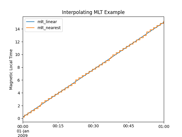
is a list of model variables that will be interpolated onto inst. By default a linear interpolation is performed but a nearest neighbor option is also supported.

# Store results for linear interpolation
inst.rename({new_data_keys[0]: "mlt_linear"})

# Run interpolation using 'nearest'
new_data_keys = pysatModels.utils.extract.instrument_view_through_model(
    inst, model.data, ['longitude'], ['longitude'], 'time', 'time',
    ['deg'], ['mlt'], ['nearest'])
inst.rename({new_data_keys[0]: "mlt_nearest"})

# Set up time range for plotting results
stime = inst.date
etime = inst.date + dt.timedelta(hours=1)

The results of

title = 'Interpolating MLT Example'
ylabel = 'Magnetic Local Time'
inst[stime:etime, ['mlt_linear', 'mlt_nearest']].plot(title=title,
                                                     ylabel=ylabel)

are shown below.

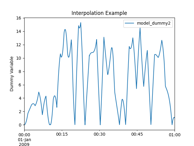
Multidimensional interpolation is performed in the same manner.

new_data_keys = pysatModels.utils.extract.instrument_view_through_model(inst,
                           model.data, ['latitude', 'longitude', 'altitude'],
                           ['latitude', 'longitude', 'altitude'], 'time',
                           'time', ['deg', 'deg', 'km'], ['dummy2'])

The

['latitude', 'longitude', 'altitude']

term provides the content and ordering of the coordinates for model variables to be interpolated. The subsequent

['latitude', 'longitude', 'altitude']

term provides the equivalent content from the satellite’s data set, in the same order as the model coordinates. The

'time', 'time'

terms cover the model labels used for time variable and coordinate. The

['deg', 'deg', 'km']

term covers the units for the model dimensions (latitude/longitude/altitude). Units for the corresponding information from inst are taken directly from the pysat.Instrument object. The final presented input

['dummy2']

is a list of model variables that will be interpolated onto inst.

The results of

    # Use the same time range as the prior example
ylabel = 'Dummy Variable'
inst[stime:etime, new_data_keys].plot(title='Interpolation Example',
                                      ylabel=ylabel)

are shown below.

Irregular Grid Models

Some models aren’t on a regular grid, or may not be a regular grid across the coordinates of interest. Consider an alternative model data set,

model = pysat.Instrument('pysat', 'testmodel', tag='pressure_levels')
model.load(2009, 1)
model.data

<xarray.Dataset>
Dimensions:       (time: 24, latitude: 72, longitude: 144, lev: 57, ilev: 57)
Coordinates:
  * time          (time) datetime64[ns] 2009-01-01 ... 2009-01-01T23:00:00
  * latitude      (latitude) float64 -88.75 -86.25 -83.75 ... 83.75 86.25 88.75
  * longitude     (longitude) float64 -180.0 -177.5 -175.0 ... 172.5 175.0 177.5
  * lev           (lev) float64 -7.0 -6.75 -6.5 -6.25 -6.0 ... 6.25 6.5 6.75 7.0
  * ilev          (ilev) float64 -6.875 -6.625 -6.375 ... 6.625 6.875 7.125
Data variables:
    uts           (time) float64 0.0 3.6e+03 7.2e+03 ... 7.92e+04 8.28e+04
    altitude      (time, ilev, latitude, longitude) float64 0.0 0.0 ... 5.84e+07
    dummy_drifts  (time, ilev, latitude, longitude) float64 0.0 0.0 ... 83.01
    slt           (time, longitude) float64 12.0 12.17 12.33 ... 10.67 10.83
    mlt           (time, longitude) float64 12.2 12.37 12.53 ... 10.87 11.03
    dummy1        (time, latitude, longitude) float64 0.0 0.0 0.0 ... 0.0 9.0

Model variables, such as dummy_drifts, are regular over (time, ilev, latitude, longitude), where ilev is a constant pressure level. Unfortunately, the observational data in inst doesn’t contain pressure level as a simulated/measured parameter. However, altitude is present in the model data but varies over all four coordinates. Interpolating dummy_drifts onto inst requires either adding an appropriate value for ilev into inst, or interpolating model variables using the irregular variable altitude instead of ilev.

Altitude to Pressure

pysatModels.utils.extract.instrument_altitude_to_model_pressure() will use information in a model to generate appropriate pressure levels for a supplied altitude in an observational-like data set.

import pysatModels

keys = pysatModels.utils.extract.instrument_altitude_to_model_pressure(inst,
            model.data, ["altitude", "latitude", "longitude"],
            ["ilev", "latitude", "longitude"],
            "time", "time", ['', "deg", "deg"],
            'altitude', 'altitude', 'cm')

The function will guess a pressure level for all locations in inst and then use the regular mapping from pressure to altitude to obtain the equivalent altitude from the model. The pressure is adjusted up/down an increment based upon the comparison and the process is repeated until the target tolerance (default is 1 km) is achieved. The keys for the model derived pressure and altitude values added to inst are returned from the function.

inst['model_pressure']

Epoch
2009-01-01 00:00:00    3.104662
2009-01-01 00:00:01    3.104652
2009-01-01 00:00:02    3.104642
2009-01-01 00:00:03    3.104632
2009-01-01 00:00:04    3.104623
                         ...
2009-01-01 23:59:55    2.494845
2009-01-01 23:59:56    2.494828
2009-01-01 23:59:57    2.494811
2009-01-01 23:59:58    2.494794
2009-01-01 23:59:59    2.494776
Name: model_pressure, Length: 86400, dtype: float64

# Calculate difference between interpolation techniques
inst['model_altitude'] - inst['altitude']

Epoch
2009-01-01 00:00:00   -0.744426
2009-01-01 00:00:01   -0.744426
2009-01-01 00:00:02   -0.744425
2009-01-01 00:00:03   -0.744424
2009-01-01 00:00:04   -0.744424
                         ...
2009-01-01 23:59:55   -0.610759
2009-01-01 23:59:56   -0.610757
2009-01-01 23:59:57   -0.610754
2009-01-01 23:59:58   -0.610751
2009-01-01 23:59:59   -0.610749
Length: 86400, dtype: float64

Using the added model_pressure information model values may be interpolated onto inst using regular grid methods.

new_keys = pysatModels.utils.extract.instrument_view_through_model(inst,
                model.data, ['model_pressure', 'latitude', 'longitude'],
                ['ilev', 'latitude', 'longitude'], 'time', 'time',
                ['', 'deg', 'deg'], ['dummy_drifts'])

inst['model_dummy_drifts']

Epoch
2009-01-01 00:00:00    30.289891
2009-01-01 00:00:01    30.305303
2009-01-01 00:00:02    30.320704
2009-01-01 00:00:03    30.336092
2009-01-01 00:00:04    30.351469
                         ...
2009-01-01 23:59:55    63.832658
2009-01-01 23:59:56    63.868358
2009-01-01 23:59:57    63.904047
2009-01-01 23:59:58    63.939724
2009-01-01 23:59:59    63.975389
Name: model_dummy_drifts, Length: 86400, dtype: float64

The time to translate altitude to model pressure is ~3 s, and the regular interpolation takes an additional ~300 ms.

Irregular Variable

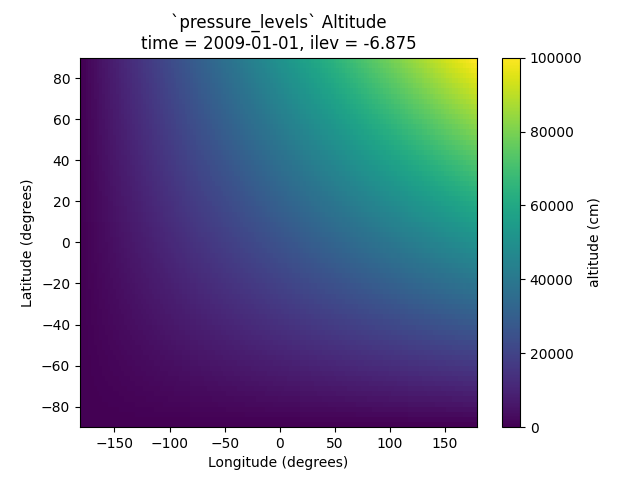
More generally, pysatModels.utils.extract.interp_inst_w_irregular_model_coord() can deal with irregular coordinates when interpolating onto an observational-like data set using scipy.interpolate.griddata(). The model loaded above is regular against pressure level, latitude, and longitude. However, it is irregular with respect to altitude.

Here is a sample distribution of the model['altitude'] for ilev=0 and the first model time.

import matplotlib.pyplot as plt

# Make base plot of 'altitude' for ilev=0 and time=0
model[0, 0, :, :, "altitude"].plot()

# Prep labels
xlabel = "".join([model.meta["longitude", model.meta.labels.name], " (",
                  model.meta["longitude", model.meta.labels.units],
                  ")"])
ylabel = "".join([model.meta["latitude", model.meta.labels.name], " (",
                  model.meta["latitude", model.meta.labels.units],
                  ")"])
cblabel = "".join([model.meta["altitude", model.meta.labels.name], " (",
                   model.meta["altitude", model.meta.labels.units],
                   ")"])

# Update labels
plt.xlabel(xlabel)
plt.ylabel(ylabel)

# Update color bar and title
fig = plt.gcf()
fig.axes[1].set_ylabel(cblabel)
fig.axes[0].set_title("".join(["`pressure_levels` Altitude\n",
                               fig.axes[0].title.get_text()]))

plt.show()

To interpolate against the irregular variable, the pysatModels.utils.extract.interp_inst_w_irregular_model_coord() function should be used. Generalized irregular interpolation can take significant computational resources, so we start this example by loading smaller pysat.Instrument objects.

inst = pysat.Instrument('pysat', 'testing', max_latitude=10.,
                        num_samples=100)
model = pysat.Instrument('pysat', 'testmodel', tag='pressure_levels',
                         num_samples=5)
inst.load(2009, 1)
model.load(2009, 1)

keys = pysatModels.utils.extract.interp_inst_w_irregular_model_coord(inst,
            model.data, ["altitude", "latitude", "longitude"],
            ["ilev", "latitude", "longitude"],
            "time", ["cm", "deg", "deg"], "ilev",
            "altitude", [50., 2., 5.],
            sel_name=["dummy_drifts", "altitude"])

# CPU times: user 419 ms, sys: 13 ms, total: 432 ms
# Wall time: 431 ms

# Print results from interpolation
inst['model_dummy_drifts']

Epoch
2009-01-01 00:00:00    22.393249
2009-01-01 00:00:01    22.405926
2009-01-01 00:00:02    22.418600
2009-01-01 00:00:03    22.431272
2009-01-01 00:00:04    22.443941
                         ...
2009-01-01 00:01:35    23.592833
2009-01-01 00:01:36    23.605252
2009-01-01 00:01:37    23.617668
2009-01-01 00:01:38    23.630081
2009-01-01 00:01:39    23.642492
Name: model_dummy_drifts, Length: 100, dtype: float64

In the interpolation function, inst and model.data provide the required data through the pysat.Instrument and xarray.Dataset objects. The

["altitude", "latitude", "longitude"]

term provides the content and ordering of the spatial locations for inst. The subsequent

["ilev", "latitude", "longitude"]

term provides the equivalent regular dimension labels from model.data, in the same order as the underlying model dimensions. While this function does operate on irregular data it also needs information on the underlying regular memory structure of the variables. The

"time"

terms cover the model label used for the datetime coordinate. The

["cm", "deg", "deg"]

term covers the units for the model information (altitude/latitude/longitude) that maps to the inst information in the coordinate list ["altitude", "latitude", "longitude"]. Note that the "cm" covers units for 'altitude' in model.data, the variable that will replace 'ilev', while the second two list elements (both "deg") covers the units for the latitude and longitude dimensions. Units for the corresponding information from inst are taken directly from the pysat.Instrument object. The

"ilev"

identifies the regular model dimension that will be replaced with irregular data for interpolation. The

"altitude"

identifies the irregular model variable that will replace the regular coordinate. The

[50., 10., 10.]

term is used to define a half-window for each of the inst locations, in units from inst, used to downselect data from model.data to reduce computational requirements. In this case a window of +/-50 km in altitude, +/-10 degrees in latitude, and +/-10 degrees in longitude is used. The keyword argument

sel_name = ["dummy_drifts", "altitude"]

identifies the model.data variables that will be interpolated onto inst. If you don’t account for the irregularity in the desired model coordinates, the interpolation results are affected.

keys = pysatModels.utils.extract.instrument_altitude_to_model_pressure(inst,
             model.data, ["altitude", "latitude", "longitude"],
             ["ilev", "latitude", "longitude"],
             "time", "time", ['', "deg", "deg"],
             'altitude', 'altitude', 'cm')
new_data_keys = pysatModels.utils.extract.instrument_view_through_model(
    inst, model.data, ['model_pressure', 'latitude', 'longitude'],
    ['ilev', 'latitude', 'longitude'], 'time', 'time', ['', 'deg', 'deg'],
    ['dummy_drifts'], model_label='model2')

# CPU times: user 3.11 ms, sys: 388 µs, total: 3.5 ms
# Wall time: 3.14 ms

# Compare interpolated `dummy_drifts` between two techniques
inst['model2_dummy_drifts'] - inst['model_dummy_drifts']

Epoch
2009-01-01 00:00:00   -0.024180
2009-01-01 00:00:01   -0.023968
2009-01-01 00:00:02   -0.023756
2009-01-01 00:00:03   -0.023544
2009-01-01 00:00:04   -0.023332
                         ...
2009-01-01 00:01:35   -0.011532
2009-01-01 00:01:36   -0.011326
2009-01-01 00:01:37   -0.011120
2009-01-01 00:01:38   -0.010914
2009-01-01 00:01:39   -0.010708
Length: 100, dtype: float64